Introduction
This was a series of labs with a culmulative experiment and design for the UofT course MIE313: Heat and Mass Transfer. I worked in a team of 4 with Muhammad Amier Mohd Faudzi, Dahlia Milevsky, Shehroz Mubashir.
My main responsibilty was to:
- create the nodal analysis and create the MATLab code to run it.
- re-derive the heat flux of the blocks, as our previous derivtions and values were incorrect.
- write the report sections that explained the code and derivations (AKA my main responsibilties).
With my group, I also:
- gathered data at all lab sessions.
- edited and formated the reports.
My group members derived and calculated the heat coefficients and other values required, as well applied the statistical analysis to validate our results.
The main objective was to find the best configuration of the two heat sinks on a circuit board with three heated aluminum blocks that minimized the maximum temperature on the circuit board.
The three blocks were fixed at specified locations on the circuit board. During lab tests, the heat sinks were placed in one of the three blocks and the temperature distribution was measured.
We experimentally gathered data on 2 configurations and simulated the same with MATLAB to validate the code.
After analyzing the simulation results, the best configuration was determined and then confirmed by experimentally testing all configurations twice.
Creating the Nodal Analysis
An analytical solution of the circuit board was created with a modified numerical method; Specifically, heat transfer was solved with a finite-difference numerical method, which solves differential equations by replacing the derivatives with an algebraic equation (or more specifically a difference).
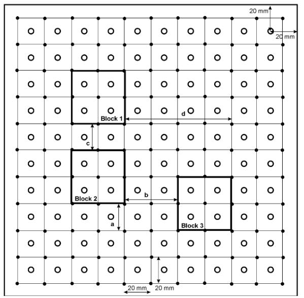 |
Two-dimensional heat conduction was used, so that the circuit board was modeled as a grid of nodes, as shown. Each circle is a node with a volume element, 20mm by 20mm. The corners of the volume element would be the holes in the circuit board. |
The temperature of each node is found under steady state conditions using an energy balance equation.
The rate of heat conduction for each side, and the rate of heat transfer through convection from the surface, was found using equations modified into finite difference forms.
The heat flux from the heater block was different for each block, and was found from the power emitted. However, the heat flux from the heater block would’ve changed if the heater block has the heat sink attached; so, it was calculated using an energy balance equation.
To account for the heat sink, its heat transfer coefficient was found using data found in a previous lab.
Nodal Analysis: Equation Derivation
In order to create the MATLAB code, first the temperature equation for each node must be made.
Normally, a 2D finite method heat transfer equation only considers the sides of the element but in this experiment the surface area of the circuit board had to be included to account for the heat flux of the heater blocks and the heat loss through combined convection and radiation.
So instead of using a more complex 3D finte method, the equation was altered so that heat travelled through a plane of each side of the element side, using the length and the element and the thickness of the circuit board.
As well, both the combined heat convection and radiation, and the heat generated from the heater block traveled through the element’s surface area.
Open below for the entire derivation.
Click to see details!
Let t be the thickness of the circuit board:
If there is no heat generation, then egen is simply 0. If there is no convection, the equation is as follows:
For the node where 1/2 of its surface area is covered by the heater block and the other 1/2 experiences convection, the temperature formula is:
For the node where a quarter of its surface area is covered by the heater block and 3/4 of its surface experiences convection:
There are three heater blocks and each has its own heat flux, which was calculated with another energy balance equation.
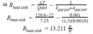
First, the thermal resistance of the heat sink is recalculated using previous lab test results and given information.
Second, the area of the hint sink was found using the dimensions provided in the data sheet [2].
Third, the heat transfer coefficient of the heat sink is calculated
Finally, the heat flux of the heater block with a heat sink is derived from an energy balance equation, where the top is to the face attached to the heat sink, the heat flux goes through the bottom to the circuit board, and Ėgen is the power emitted from the heater block.
If the heater block does not have the heat sink attached, then hconv is replaced with hblock:
MatLab Code
Equations (1) to (6) and parameters - either calculated in the above collapsible, provided from the Lab manual or from Table 2 - were used in a MATLAB m-file using the Gauss-Seidel numerical method to solve the temperature of each node.
Credit to my classmates and the TAs who helped me figure out MatLab coding, and how to properly format the equations. I was at my limit with my temperature.m file.
config.m provided two matrices, one that marked which element required which equation, and another to indicate which heater block had a heat sink.
Click to see config.m code!
    function [circuitboard, heatsinks] = config(n)
    %n is the given input from 1-3, output the corresponding matrix

    circuitboard = zeros(11,11);
    %0 convection 1 quater 2 half 3 full 4 quarter 5 half 6 full 7 quater 8 half 9 full

    %full egen
    %first block            second block          third block
    circuitboard( 4,6)=3; circuitboard (7,5)=6; circuitboard (8,8)=9;

    %half egen
    %first block            second block          third block
    circuitboard (3,6)=2; circuitboard (6,5)=5; circuitboard (7,8)=8;
    circuitboard (5,6)=2; circuitboard (8,5)=5; circuitboard (9,8)=8;
    circuitboard (4,5)=2; circuitboard (7,4)=5; circuitboard (8,7)=8;
    circuitboard (4,7)=2; circuitboard (7,6)=5; circuitboard (8,9)=8;

    %quater egen
    %first block            second block          third block
    circuitboard (3,5)=1; circuitboard (6,4)=4; circuitboard (7,7)=7;
    circuitboard (3,7)=1; circuitboard (6,6)=4; circuitboard (7,9)=7;
    circuitboard (5,5)=1; circuitboard (8,4)=4; circuitboard (9,7)=7;
    circuitboard (5,7)=1; circuitboard (8,6)=4; circuitboard (9,9)=7;

    %output of the heat position
    heatsinks=zeros(1,3);

    %1 = heater block 1 and 2
    if n == 1
        heatsinks(1,1)=1;
        heatsinks(1,2)=1;

    %2 = heater block 1 and 3
    elseif n == 2
         heatsinks(1,1)=1;
         heatsinks(1,3)=1;

    %3 = heater block 2 and 3
    elseif n == 3
         heatsinks(1,2)=1;
         heatsinks(1,3)=1;
    End
temperaturemaker.m solved the temperature equations with Gauss-Seidel.
Click to see config.m code!
    function [tn] = temperaturemaker(flag, sink)
    % DESIGN LAB heat transfer finite method analysis of a circuit board

    %flag - 11x11 matrix inidicating what type of node
    %sink - indicates which heater has a heat sink

    max_iter = 200; %maximum # of iterations for the Gauss-Seidel
    stop = 1; % if the difference summation is less, exit

    row = 11; %
    col = 11; % row and col of the triangle only, using symmetry
    to = zeros(row,col); %the previous iteration

    k = 8.72; % k of the board
    h_normal = 10; % combined convection and radiation h of the board
    A = 0.02*0.02 - pi*0.004*0.004; % surface area of the element
    t = 0.00157; %thickness of the circuit board
    tamb = 22; %temperature of the air in celcius

    den = 4*k*t + h_normal*A; % denominator of the equations
    den50 = 4*k*t + 0.5*h_normal*A; % 50% conv, 50% egen
    den25 = 4*k*t + 0.75*h_normal*A; % 75% conv, 25% egen

    %%% Egens = V^2/@RArea of heater block
    V2 = (24.5*24.5);
    R = [81.4 77.7 78.7];  % heater block's resistances

    A_face = 0.0016; % heater block's surface area of the top and bottom
    A_side = 0.01*0.04*4; % heater block's surface area of all 4 sides

    h_heatsink = 33.064594; %convection coef of the heat sink
    T_heatsink = (87.2+89.9)/2; % avg surface temp of the heater block to the heat sink
    egen = zeros(1,3); % the egen of the heater block, index corrospond to heat block #

    % calculate the egens based on # and if they have a heat sink
    for i=1:3
        if sink(i) == 1 %it has the heat sink attached
            egen(i) = V2/(R(i)*A_face) - (T_heatsink - tamb)*(h_heatsink + h_normal*(A_side/A_face) )  ;

        else %it does NOT have the heat sink
            egen(i) = V2/(R(i)*A_face) - h_normal*(T_heatsink - tamb)*(1+(A_side/A_face) );
        end
    end
    %%% END Egens

    %%% INITILIZE - set temperature boundary conditions
    %top row temperatures
    to(1,1) = 26.8; to(1,2) = 29; to(1,3) = 27.7;
    to(1,4) = 27.5; to(1,5) = 27.7; to(1,6) = 26.2;
    to(1,7) = 28.2; to(1,8) = 29.6; to(1,9) = 29.7; to(1,10) = 29.4;
    % right column tempertatures
    to(1,11) = 28.8; to(2,11) = 28.3;  to(3,11) = 28;
    to(4,11) = 28.4; to(5,11) = 29.4; to(6,11) = 30.6;
    to(7,11) = 31.5; to(8,11) = 33.3; to(9,11) = 34.8;  to(10,11) = 35;
    % bottom row tempertatures
    to(11,2) = 30.9; to(11,3) = 31.5; to(11,4) = 32.4;
    to(11,5) = 32.6; to(11,6) = 32.3; to(11,7) = 32.3;
    to(11,8) = 32.8; to(11,9) = 32.8; to(11,10) = 33.4; to(11,11) = 34.5;
    %left column temperatures
    to(2,1) = 26.8; to(3,1) = 26.1; to(4,1) = 25.9;
    to(5,1) = 26.1; to(6,1) = 27.9; to(7,1) = 27.7;
    to(8,1) = 27.4; to(9,1) = 27.1; to(10,1) = 27.4; to(11,1) = 28.4;
    %%% END INITILIZE - set temperature boundary conditions

    tn = to; % create the matrix that will store the current iteration

    %%% FINITE DIFFERENCE METHOD SOLUTION WITH GAUSS SEIDEL
    iter = 1; % counts the # of iterations

    %egen = new_egen-egen
    while iter < max_iter %keeps iterating until max

        for i=2:(row-1) % skip the boundary border nodes
            for j=2:(col-1)

                if flag(i,j) == 0 %no egen, w/ convection
                    tn(i,j) = (1/den)*( (k*t)*(to(i,j-1)+to(i+1,j)+to(i,j+1)+to(i-1,j)) + (h_normal*A)*tamb ) ;
                % heater block 1
                elseif flag(i,j) == 3 % all egen
                    tn(i,j) = 0.25*( (to(i,j-1)+to(i+1,j)+to(i,j+1)+to(i-1,j)) + egen(1)*(A/k*t) );
                elseif flag(i,j) == 1 %25% egen, 75% convection
                    tn(i,j) = (1/den25)*((k*t)*(to(i,j-1)+to(i+1,j)+to(i,j+1)+to(i-1,j))+ egen(1)*(A*0.25) + (h_normal*A*0.75)*tamb );
                elseif flag(i,j) == 2 %half egen, half convection,
                    tn(i,j) = (1/den50)*((k*t)*(to(i,j-1)+to(i+1,j)+to(i,j+1)+to(i-1,j))+ egen(1)*(A*0.5) + (h_normal*A*0.5)*tamb );
               % heater block 2
                elseif flag(i,j) == 6 % all egen
                    tn(i,j) = 0.25*( (to(i,j-1)+to(i+1,j)+to(i,j+1)+to(i-1,j)) + egen(2)*(A/k*t) );
                elseif flag(i,j) == 4 %25% egen, 75% convection
                    tn(i,j) = (1/den25)*((k*t)*(to(i,j-1)+to(i+1,j)+to(i,j+1)+to(i-1,j))+ egen(2)*(A*0.25) + (h_normal*A*0.75)*tamb );
                elseif flag(i,j) == 5 %half egen, half convection,
                    tn(i,j) = (1/den50)*( (k*t)*(to(i,j-1)+to(i+1,j)+to(i,j+1)+to(i-1,j)) + egen(2)*(A*0.5) + (h_normal*A*0.5)*tamb );
                % heater block 3
                elseif flag(i,j) == 9 % all egen
                    tn(i,j) = 0.25*( (to(i,j-1)+to(i+1,j)+to(i,j+1)+to(i-1,j)) + egen(3)*(A/k*t) );
                elseif flag(i,j) == 7 %25% egen, 75% convection
                    tn(i,j) = (1/den25)*((k*t)*(to(i,j-1)+to(i+1,j)+to(i,j+1)+to(i-1,j))+ egen(3)*(A*0.25) + (h_normal*A*0.75)*tamb );
                elseif flag(i,j) == 8 %half egen, half convection,
                    tn(i,j) = (1/den50)*( (k*t)*(to(i,j-1)+to(i+1,j)+to(i,j+1)+to(i-1,j)) + egen(3)*(A*0.5) + (h_normal*A*0.5)*tamb );

                end % end ifs
            end % end col for
        end% end row for

        difsum = sum(sum(abs(to-tn))); % Calculate the difference summation
        if difsum < stop %check stop condition
            max_iter = iter;
            break;
        end

        to=tn; %update the matrix storing previous iteration
        iter = iter+1; %increase the counter

    end % End of the while loop/Gauss-Seidel iteration
main.m found which configuration had the lowest maximum temperature, calling on the config to create the blocks and temperature files to solve the temp distribution.
Click to see main.m code!
    %main function: Finds the config which has the lowest max temp
    %calling configuration function for the configurations of the blocks
    [circuitboard,heatsinks] =config(1); % heater block 1 and 2

    %send the matrix to the temperature function to get the temperature
    %distribution
    temp1 =temperaturemaker(circuitboard,heatsinks);

    %find max temp in the matrix
    [row,column]=size(circuitboard);
    max = 200;
    store = 0;
    max_temp1=0;
    max_temp2=0;
    max_temp3=0;
    index = [0,1,2]; %[row, col]

    for i=1:row;
        for j=1:column;
            if temp(i,j)>max_temp1
                max_temp1 =temp(i,j);
                index = [1,i,j];
            end
        end
    end

    if max>max_temp1
        best_configuration=temp1;
        max = max_temp1;
        store = index;
    end

    %call configuration for second location and repeat
    [matrix2a,matrix2b] =config(2); % heater block 1 and 3
    temp2 =temperaturemaker(matrix2a,matrix2b);
    for i=1:row;
        for j=1:column;
            if temp2(i,j)>max_temp2
                max_temp2=temp2(i,j);
                index = [2,i,j];
            end
        end
    end

    if max>max_temp2
        best_configuration=temp2;
        max = max_temp2;
        store = index;
    end

    %call configuration for third location
    [matrix3a, matrix3b] =config(3); % heater block 2 and 3
    temp3 =temperaturemaker(matrix3a,matrix3b);
    for i=1:row;
        for j=1:column;
            if temp3(i,j)>max_temp3
                max_temp3=temp3(i,j);
                index = [3,i,j];
            end
        end
    end

    if max>max_temp3
        best_configuration=temp3;
        max = max_temp3;
        store = index;
    end
Results and Analysis
There were 3 possible configurations, the heat sinks places on:
- heating block 1 and 2
- heating block 1 and 3
- heating block 2 and 3
MatLab Results
Config 1 was tested and then used to validate the MatLAb simulation already created. Afterwards, config 3 was also tested to validate its results.
The parameters were as followed:
| Ambient Temp. |
Block 1 Heat Resistance |
Block 2 Heat Resistance |
Block 3 Heat Resistance |
Applied Voltage |
Block 1 Temp. |
Block 2 Temp. |
Block 3 Temp. |
|
|---|---|---|---|---|---|---|---|---|
| Value | 22 °C | 81.4 Ω | 77.7 Ω | 87.0 Ω | 24.5 V | 87.2 °C | 100.9 °C | 89.9 °C |
The following chart compares the Matlab results to the Lab results:
| MatLab | MatLab | Lab 1 | Lab 1 | |
|---|---|---|---|---|
| Max. Temp. | Coordinate | Max. Temp. | Coordinate | |
| Config. 1 | 80.70 °C | (8,7) | 78.1 °C | (6,4) |
| Config. 2 | 85.14 °C | (7,6) | N/A | N/A |
| Config. 3 | 80.09 °C | (5,6) | 68.8 °C | (7,7) |
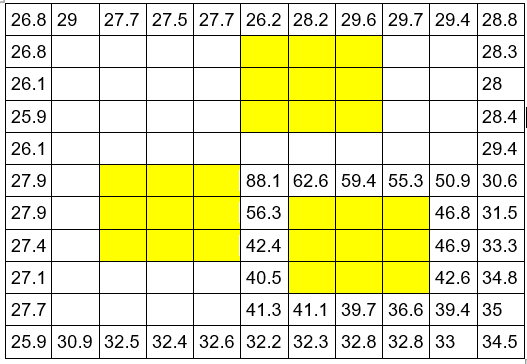
The follwing images shows the recorded data from lab 1:
| Lab 1 Config 1 | Lab 1 Config 2 |
|---|---|
 |
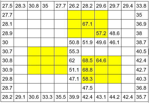 |
The yellow squares show where the blocks were placed. As seen below, all perimeter nodes were recorded, as well were the center nodes and others of interest.
| Configuration 1 Comparison: Experimental vs MatLab | |
|---|---|
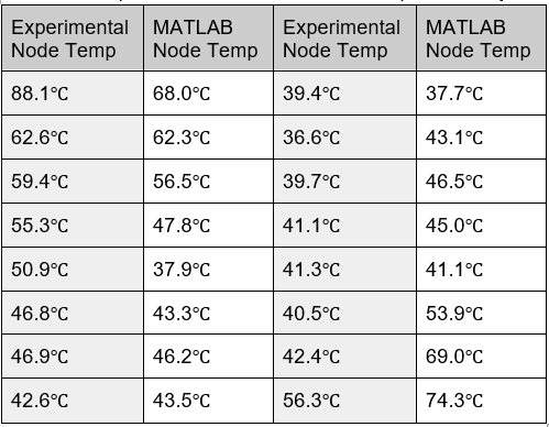 |
MatLab had significant difference for config three, but only for what it calculated was the highest temperature and its location. The error most likely is the convention values or how they were applied in the equations. In Matlab, the hottest node was exposed in the air and situated in the center of 3 heating blocks. However, the lab results show the hottest node was under a block. |
In addition, errors can be attributed to the fact several assumptions were taken while conducting the analytical technique like 2D heat transfer, constant thermal properties and convection heat transfer.
Also, heat block of different resistance is used and the inconsistencies in measuring the temperature affects our maximum temperature in configuration 3 and its location in the second lab session, hence the variation between the two lab sessions.
Lab 2 Experimental Results
The parameters of lab 2 were as followed:
| Parameter | Ambient Temp. |
Block1 Heat Resistance |
Block2 Heat Resistance |
Block3 Heat Resistance |
Applied Voltage |
Block1 Temp. |
Block2 Temp. |
Block3 Temp. |
|---|---|---|---|---|---|---|---|---|
| Value | 22 °C | 85.0 Ω | 86.0 Ω | 79.0 Ω | 24.5 V | 99.0 °C | 087.7 °C | 84.1 °C |
The table below show the highest temperatures recorded in each configuration during lab 2:
| Max. Temp. | Coordinate | |
|---|---|---|
| Config. 1 | 80.66 °C | (8,7) |
| Config. 2 | 80.52 °C | (7,6) |
| Config. 3 | 76.45 °C | (6,4) |
| Configuration 3 Comparison: Experimental vs MatLab | |
|---|---|
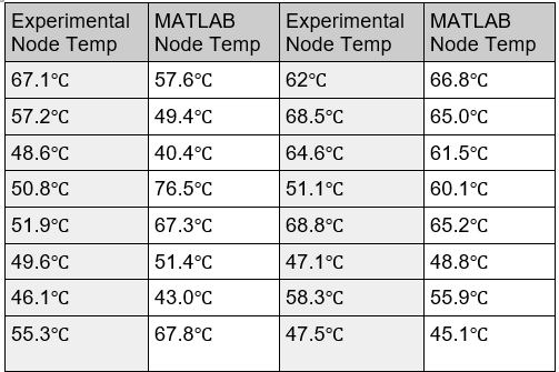 |
The results were similar to lab1. This confirmed that config 3 was the best, and that our MatLab simulation was correct. |
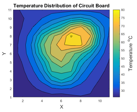
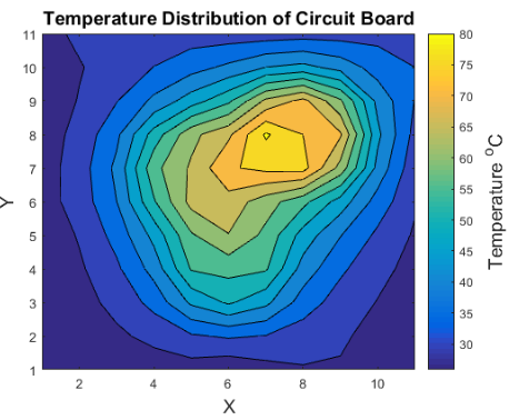
The following are graphs made on MatLab of the heat distributions from the 2 additional tests done in lab 2:
| Test 1 | Test 2 | |
|---|---|---|
| Config 1 |
 |
 |
| Config 2 |
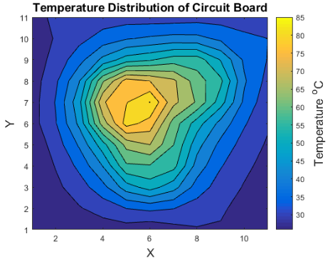 |
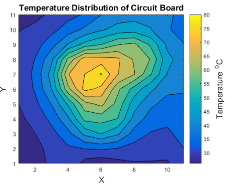 |
| Config 3 |
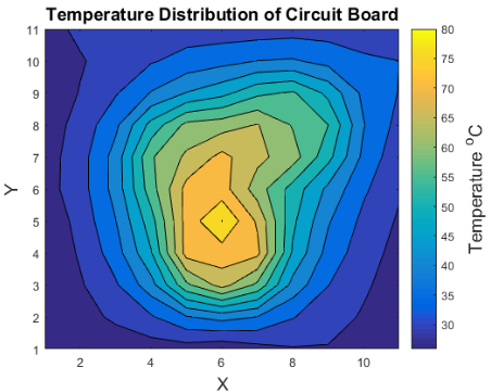 |
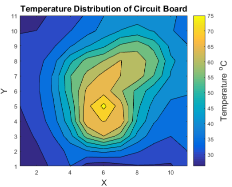 |
Conclusion
We concluded that config 3 - heat sinks on blocks 2 and 3 - was the optimal placement.
Changes and Recommendations
We recommended that a larger number of iterations should’ve been used in the finite difference to minimize variances and that heat blocks of similar resistance should’ve been used in the experiments.
We would’ve also prefered a better technique of positioning the aluminum blocks on the circuit board.
For example, border lines around the nodes on the circuit board as seen in figure 1, or even snap fit connection between blocks and circuits as the blocks were easily moved due to the equipment and wires connected to it.
Notes:
Mostly complete. Just needs final format/edits. Maybe of images of the physical things.


